I’m a mechanical engineer, but my job involves both research and testing. To that point, I often work with large amounts of data. Last week, I ran into a fun problem that required a more sophisticated analytical model than I was used to building. That’s what makes research fun! It also gave me a chance to finally explore scikit-learn and familiarize myself with the Random Forests algorithm.

Problem Definition

In a general sense, I was trying to build a model that would take measured data and determine an outcome based on the measurements. In other words, a model. However, I wanted to know exactly which measurements were the most influential in ultimately determining the outcome.

After reading around, it seemed that the Random Forest algorithm is often used for determining input importance. Although, from what I can tell, the algorithm isn’t used very often in the physical sciences. One reason is likely the fact that Random Forests is still fairly new; it only dates back to 2001 when Leo Breiman, a statistician at the University of California, Berkeley authored this extremely well-cited paper.

I want to keep the tone of this post practical rather than theoretical, so I won’t be delving into any math. However, if you’re looking for more background information on the topic, I’d recommend the following lectures/talks that have graciously uploaded to Youtube:

Machine learning – Random forests by Nando de Freitas
Random Forests Theory and Applications for Variable Selection by Hemant Ishwaran

These Youtube lectures are great, but they don’t really help in building an actual functioning model. Fortunately, a group of smart people have put together a truly outstanding library for Python called scikit-learn. It’s capable of doing all the leg work of implementing a Random Forest model, and much, much more. As awesome as scikit-learn is, I found their examples for to be a overwhelming. I also struggled to find any “dumbed down” examples anywhere other than here. That post includes a short code example, but it doesn’t include annotations or comments. The authors produced a handful of useful plots, but didn’t explain how they produced those, either. I’ll use this opportunity to pick up where they left off!

Create Random Forests Test/Training Sets

If you jumped ahead, what we’re about to do is analyze a dataset that includes several measurements of flowers. Then, we’re going to predict the species of each flower, based on their measurements. If this is your first time working with scikit-learn, make sure it’s available to your environment since it’s not a standard library.

The first line imports the Random Forest module from scikit-learn. The next pulls in the famous iris flower dataset that’s baked into scikit-learn. Numpy, pandas, and matplotlib are all libraries that are probably familiar to anyone looking into machine learning with Python.

from sklearn.ensemble import RandomForestClassifier as RFC
from sklearn.datasets import load_iris

import numpy as np
import pandas as pd
import matplotlib.pyplot as plt

We’ll go ahead and assign the load_iris module to a variable, and use its methods to returning data required to construct a pandas dataframe.

iris = load_iris()
df = pd.DataFrame(iris.data, columns=iris.feature_names)

I’m assuming the reader is familiar with the concepts of training and testing subsets. To create said sets, we create a (random) uniform distribution between 0 and 1. We then assign 3/4ths of the data to the training subset.

df['is_train'] = np.random.uniform(0, 1, len(df)) <= .75

This is a portion of the code that I had to adapt from the yhat example. Evidently, the factor method used in the yhat example has been developed since their post, and was at some point renamed. In any case, this from_codes method takes an array of numbers (iris.target) and associates those numbers (as indices) with the second array to build a new array that’s composed entirely of the second array’s values. I tend to think of this as “decompressing” the data. We’re going to undo this momentarily, but everything up to this point has been an attempt to mimic a real-world dataframe.

df['species'] = pd.Categorical.from_codes(iris.target, iris.target_names)

The training and test sets are now explicitly split into their own dataframes, and “features” are defined. Features are essentially just the model’s input variables.

train, test = df[df['is_train']==True], df[df['is_train']==False]
features = df.columns[0:4]

Run the Random Forests Model

Next, a Random Forest class is established with just 2 arguments. The number of jobs n_jobs are irrelevant for this simple problem, but the argument essentially dictates how much processing power to use. The second argument isn’t included in the yhat example, but it specifies how many decision trees to include in the forest. It should be noted that more trees does not mean the process will create a more-correct model.

forest = RFC(n_jobs=2,n_estimators=50)

Remember the “decompression” we did a few lines back? Well, we’re going to recompress it again. Up to this point, the species were verbosely defined in the array as “setosa”, “virginica”, and “versicolor”. These categorical strings don’t necessarily make sense to our algorithm, but integers that represent each of these categories do! This is a common technique in machine learning in general, not just within this Random Forests example.

y, _ = pd.factorize(train['species'])

Now it’s time to fit our model to the measured (training) data and use it to predict the species for each of the measured (test) flowers! Lastly, a pandas module is used to spit out a table that compares the actual species from the testing subset with the species determined by the model.

forest.fit(train[features], y)
preds = iris.target_names[forest.predict(test[features])]
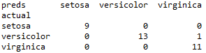
print pd.crosstab(index=test['species'], columns=preds, rownames=['actual'], colnames=['preds'])

Random Forests Results

My output is below. Remember, your results will likely not mirror mine as the Random Forest algorithm is a stochastic process. In this case, the model correctly predicted 9 stetosas and 13 versicolors. It also predicted there to be 12 virginicas, but unfortunately there were only 11. One was actually a versicolor.

There are a number of ways to represent this result. Namely, a confusion matrix or an ROC chart to name a few. Instead, I want to go back and focus on the fact that what I really wanted out of this process was to determine which variables had the greatest impact on the prediction. What I want to know is feature importance!

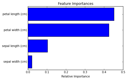
The yhat post showed this easy-to-read bar graph that compared their model’s various features’ importance, but didn’t show the code behind it.

Creating a Plot

The code for determining and graph the features’ importance is straight forward to those familiar with matplotlib. In fact, there is actually a pretty good example for this sort of graph from the official documentation. However, since this entire post builds off of the yhat example, I’ll do my best to replicate their exact result. The only tricky thing about producing this graph is that the feature_importances_ method returns the quantified relative importance in the order the features were fed to the algorithm. To make the plot pretty, we’ll instead sort the features from most to least important.

importances = forest.feature_importances_
indices = np.argsort(importances)

The only thing left to do is make the plot!

plt.figure(1)
plt.title('Feature Importances')
plt.barh(range(len(indices)), importances[indices], color='b', align='center')
plt.yticks(range(len(indices)), features[indices])
plt.xlabel('Relative Importance')

I realize I didn’t explain how the importance numbers are derived, but regardless, the results show that petal length and petal width are generally the best indicators of the flowers’ species.

Completed Code

If you’re the type of person that always skips the explanation and digs straight into the finished code example, here you go!

#Modified from the example written by yhat that can be found here:
#http://blog.yhathq.com/posts/random-forests-in-python.html

from sklearn.ensemble import RandomForestClassifier as RFC
from sklearn.datasets import load_iris

import numpy as np
import pandas as pd
import matplotlib.pyplot as plt

iris = load_iris()
df = pd.DataFrame(iris.data, columns=iris.feature_names)
df['is_train'] = np.random.uniform(0, 1, len(df)) <= .75
df['species'] = pd.Categorical.from_codes(iris.target, iris.target_names)

train, test = df[df['is_train']==True], df[df['is_train']==False]
features = df.columns[0:4]

forest = RFC(n_jobs=2,n_estimators=50)
y, _ = pd.factorize(train['species'])
forest.fit(train[features], y)

preds = iris.target_names[forest.predict(test[features])]
print pd.crosstab(index=test['species'], columns=preds, rownames=['actual'], colnames=['preds'])

importances = forest.feature_importances_
indices = np.argsort(importances)

plt.figure(1)
plt.title('Feature Importances')
plt.barh(range(len(indices)), importances[indices], color='b', align='center')
plt.yticks(range(len(indices)), features[indices])
plt.xlabel('Relative Importance')